ECCV 2026 · The 2nd UoM-SeoulTech International Joint Workshop

Not All Prediction Targets Keep
Training-Free Diffusion Guidance
on the Manifold

Presented by Hyeongmin Lee

ViViD Lab · Dept. of Electronic Engineering, SeoulTech · Aug 20, 2026

Code · github.com/ManLuML/on-manifold-tfg

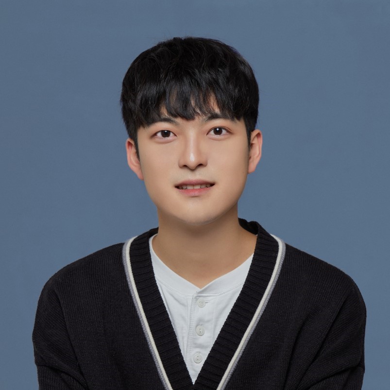
About the speaker

Hyeongmin Lee

Assistant Professor · SeoulTech, Electronic Engineering

2018 – 2023 Yonsei University · Ph.D., Electrical & Electronic Engineering
2021 Adobe Research · research intern · video stabilization
2023 – 2026 Twelve Labs · ML research scientist · video foundation models
2026 – SeoulTech · assistant professor · ViViD Lab

ViViD Lab · est. 2026

Vision and Video Dynamics Lab

Video-centric computer vision, from pixels to world models.

Video Processing

low-level video enhancement

Video Understanding

temporal semantics · representation

3D / 4D Vision

reconstruction · rendering

World Models

generative simulation of the visual world

Today's paper sits where generation meets control · steering image generators at inference time.

vivid.seoultech.ac.kr

Background · 01

Generative models

You have already used one. ChatGPT, Gemini, any image generator.

Draw a portrait of a person who does not exist.

AI

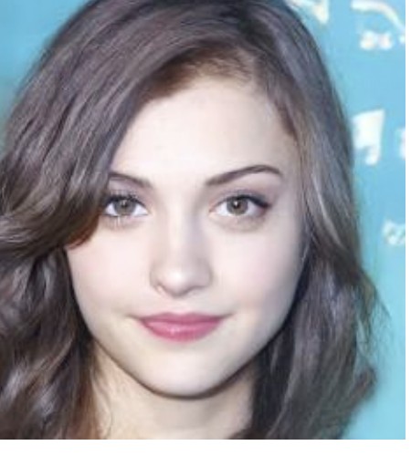
This person does not exist · the model drew her.

Reply image: a diffusion-model sample (Ho et al., NeurIPS 2020, Fig. 1) · chat window: illustrative mock-up, not a real product

Background · 02

Behind the chat window

A model that learned the distribution of real photographs, and draws new samples.

x \sim p_{\text{data}}(x)

Generated samples from DDPM: faces and CIFAR10

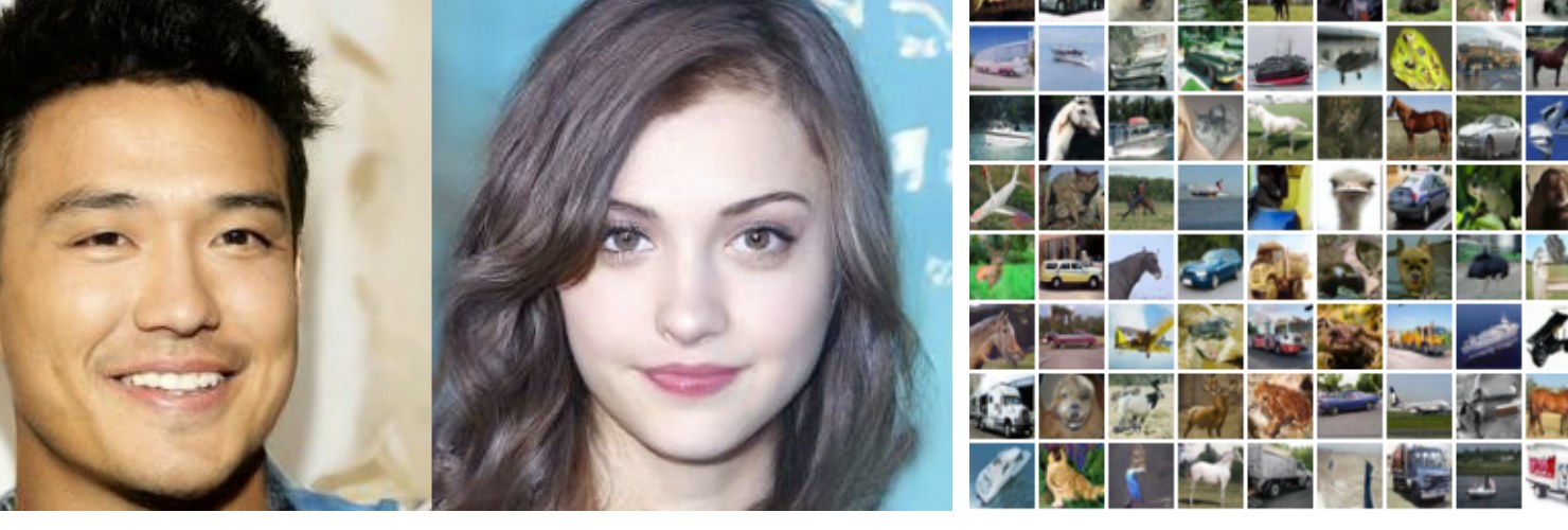
none of these people or objects exist · every image here is a model sample

Samples from a diffusion model (Ho et al., NeurIPS 2020, Fig. 1)

Background · 03

Denoising

A network that fills in what noise destroyed.

noisy photo

→

denoiser

a neural network

→

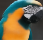
restored photo

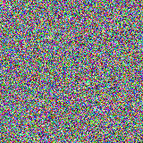
What if the input is 100% noise?

Photo crops: Li & He 2025, Fig. 7 (noisy input · restored by an x-prediction denoiser)

Background · 04

Diffusion: repeated denoising

Start from pure noise. Denoise a little, hundreds of times. An image appears.

Diffusion chain from noise x_T to image x_0

Progressive generation, noise to image, left to right

x_{t-1} \;=\; \tfrac{1}{\sqrt{\alpha_t}}\Bigl(x_t \;-\; \tfrac{1-\alpha_t}{\sqrt{1-\bar{\alpha}_t}}\,\epsilon_\theta(x_t,\,t)\Bigr) \;+\; \sigma_t\, z

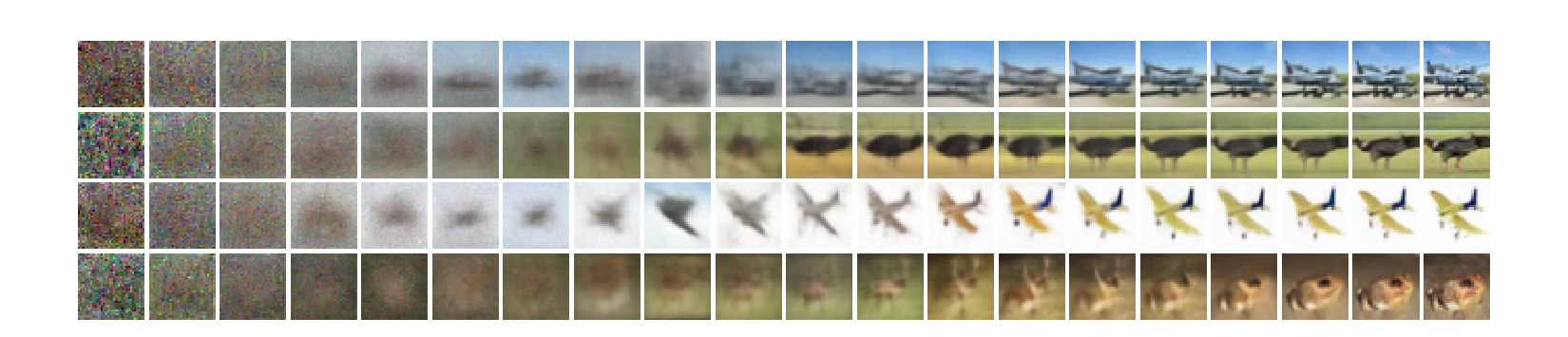
one denoising step, written out (Ho et al., 2020, Alg. 2) · no need to read it — the pictures say the same thing

Figures: Ho et al., NeurIPS 2020 (Figs. 2, 6) · sampling proceeds left to right

Background · 05

The network's output: noise

One denoising step, up close.

noisy image $z_t$

→

network

\epsilon_\theta

→

predicted noise $\hat{\epsilon}$

−

subtract
a little

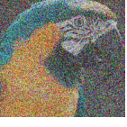
cleaner · repeat

the same step, as a formula · $\epsilon_\theta(z_t) \approx \epsilon$ · look at the noisy image, predict the noise inside it

The model never outputs an image. It outputs noise.

$\epsilon$ -prediction, the standard choice since DDPM (Ho et al., 2020) · a third target, velocity $v$ , exists but is not covered in this talk · photo crops: Li & He 2025, Fig. 7

Setting · 01

A model that draws only birds

Trained models draw random images, of anything. What if we want one class?

ImageNet
model

general

→

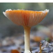
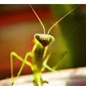
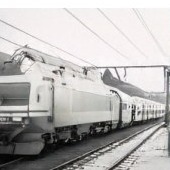
the same
model

condition · "bird"

→

How do we get the second row, without training a bird model?

All images are real model outputs · top: ImageNet samples, JiT-H (Li & He 2025, Fig. 5) · bottom: guided bird samples from our experiments (Fig. 7c)

Setting · 02

Generating only what you want

Think of every image as a point. The model samples from the whole set.

Sampling drops a point anywhere in the big set · we want it to land only in the small one.

option 1 · retrain on the subset

works, but one full training run for every new goal

option 2 · keep the model frozen, steer it

all we need is something that knows the subset

Setting · 03

A classifier knows the direction

It is a neural network. Gradients flow all the way back to the pixels.

input image $x$

→

classifier

a neural network

→

"bird" · 3%

run the gradient back to the input · $\nabla_x \log p(\text{bird}\,|\,x)$ · "how should the pixels change, to look more like a bird?"

"wings should appear" "a beak, over here" "feathers, not a cap"

not just a judge · a compass · and classifiers for almost anything are already on the shelf

Setting · 04

Training-free guidance (TFG)

Sampling walks a point from noise into the image set. Nudge every step.

one guidance step · $z \;\leftarrow\; z \;+\; \rho\,\nabla \log p(y\,|\,\htmlClass{hl}{\hat{x}_0})$

one detail · the classifier reads $\hat{x}_0$ · a clean-image estimate, not the noisy point itself

frozen model · no retraining any objective class · style · inverse problems

Shown: gradient guidance in DPS form (Chung et al., ICLR 2023) · the TFG framework (Ye et al., NeurIPS 2024) unifies these variants under one interface

The catch · 01

A classifier that has never seen noise

What happens when we hand it the middle of sampling?

→

classifier

→

"bird" · 97%

a photograph · knows exactly what to say

→

classifier

→

" ? ? ? "

nothing it was ever trained on

Trained on photographs · a noisy state is not a photograph ·
its "direction" here means nothing.

Confidence numbers are illustrative · left images: model samples and a noised state (sources as before)

The catch · 02

Where images live: a thin manifold

The same fact, drawn as a picture.

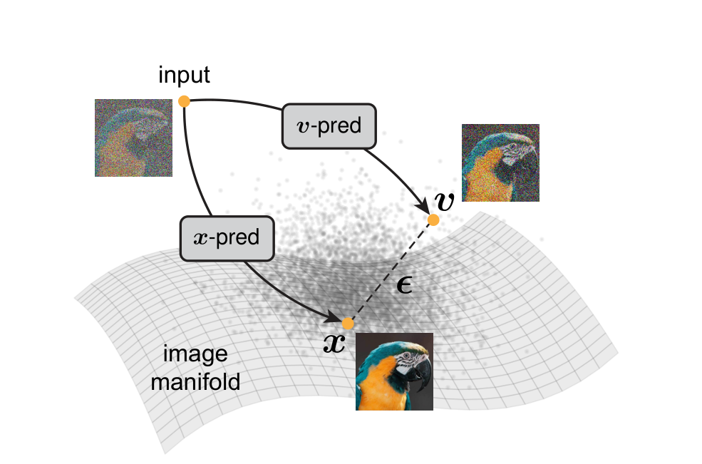
Image manifold: clean image on the surface, noised quantities off it

Li & He, arXiv:2511.13720, Fig. 1

Natural images occupy a low-dimensional manifold $\mathcal{M}$ inside pixel space.

The classifier was trained on $\mathcal{M}$ only · the noisy $z_t$ lies off $\mathcal{M}$ .

So guidance must be computed on a clean-image estimate $\hat{x}_0$ · and now everything depends on how good that estimate is.

Figure labels $v$ (velocity), a third prediction target omitted in this talk · the off-manifold argument applies to every noised quantity

The weak link

Getting a clean image, mid-sampling

The classifier needs a clean image. Does the ε-model have one to give?

Tweedie's formula

\hat{x}_0 \;=\; \bigl(z_t - (1-t)\,\hat{\epsilon}\bigr)\,/\;t

predicted noise $\hat{\epsilon}$

noisy $z_t$

▸

estimate $\hat{x}_0$

draw the line from $\hat{\epsilon}$ through $z_t$ · extend it, and you land on $\hat{x}_0$

at high noise the extension is long · a small error in $\hat{\epsilon}$ lands far off · the estimate comes out damaged (~×9 near the start)

Guidance matters most at early, high-noise steps ·
exactly where this estimate is worst.

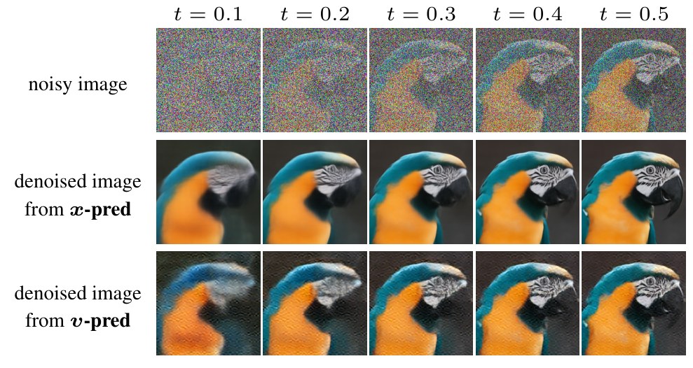
Noisy image, clean image predicted directly, clean image recovered by conversion

top · the noisy input

middle · a clean image, predicted directly by a network

bottom · a clean image, recovered by conversion · artifacts

Exact form (linear schedule): recovery divides the de-noised residual by the signal level, amplifying the network error by (1−t)/t — Prop. 1 (Eq. 1) of our paper; posterior-mean recovery, the flow-matching analogue of Tweedie's formula (Efron, 2011) · images: Li & He 2025, Fig. 7 · the recovered example converts from the velocity target, the mildest indirect case; noise-prediction is less stable still (≈3× higher training loss, ibid. §B.1)

The fix

JiT: predict the clean image instead

Just image Transformers (Li & He, 2025). The only change: what the network predicts.

noisy image

→

network · $\epsilon_\theta$

trained to predict noise

→

the noise

→

subtract
a little

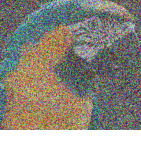
next state

the same image

→

network · $x_\theta$ · JiT

trained to predict the clean image

→

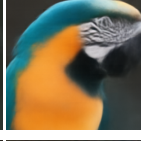
the clean image

→

step toward it
a little

the same next state

Either way, one step lands in the same place · only the network's direct output differs.

But now a clean image exists at every step · exactly what the classifier needs.

JiT: a plain ViT on pixel patches · generation quality comparable (ImageNet 256×256 FID 1.86 vs DiT-XL/2 2.27, Tab. 1 of our paper) · the targets are interconvertible parameterizations of the same step (Li & He, Tab. 1); what differs is what the network must represent · a third target, velocity, omitted · images: Li & He 2025, Fig. 7 crops

Our paper · ECCV 2026

The same recipe, two prediction targets

Frozen model + bird classifier + TFG. Only the prediction target differs.

$x$ -prediction · JiT

diverse poses · diverse backgrounds

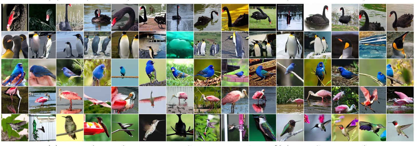
JiT under strong guidance: diverse poses and backgrounds

$\epsilon$ -prediction · DiT

the same pose, again and again · dark backgrounds

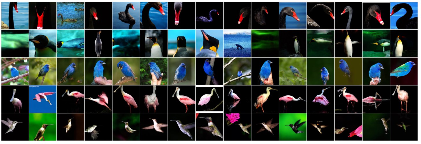
DiT under strong guidance: mode collapse, repeated poses, dark backgrounds

This is our paper's message · the prediction target decides whether guidance works.

Fig. 7(c)(d) of our paper · five species, 15 random samples each, no cherry-picking · strong guidance

Our paper · measured

Child FID: putting a number on it

C-FID · distance between guided samples of a class and real photos of that class.

Standard metrics miss the damage · classifier accuracy rewards adversarial-like images that fool the network · C-FID asks instead: do the samples look like the real class?

143 bird species 64 samples per species 9,152 images per point

At matched classifier accuracy · C-FID 32.9 ( $x$ , JiT) vs. 38.1 ( $\epsilon$ , DiT)

and a 131M x-prediction model sustains lower C-FID than a 724M $\epsilon$ -prediction model

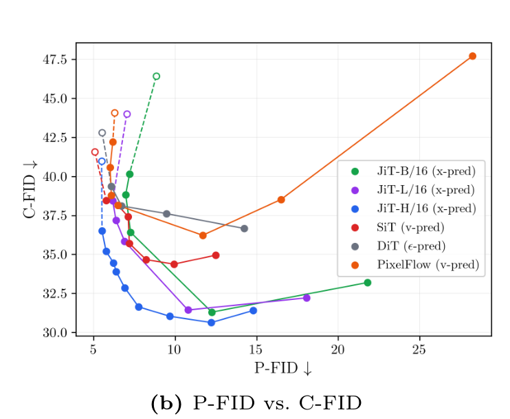
lower-left is better · $x$ -prediction keeps improving where the others reverse (Fig. 4b)

Validity: top-1 accuracy of an evaluation classifier kept separate from the guidance classifier (§4.3–4.4) · matched point ≈26.6% Validity · parameter counts include the 49M VAE decoder used at every guidance step (Tab. 1) · controlled toy ablation in the paper: at D=512, on-manifold rate 93.3% (x) vs 0.5% (ε)

Our paper · for reference

Why it works: statements and proofs

Each result with its proof, from §3 and Appendix B. Kept here for the curious reader.

Proposition 1 · Error Amplification

Let $\delta_\epsilon = \|\epsilon-\epsilon_\theta\|_2$ , $\;\delta_x = \|x-x_\theta\|_2$ . Then

\bigl\|\hat{x}^{(\epsilon)}-x\bigr\|_2 = \tfrac{1-t}{t}\,\delta_\epsilon\,, \qquad \bigl\|\hat{x}^{(x)}-x\bigr\|_2 = \delta_x

Proof. Substitute the forward process $z_t = t\,x + (1-t)\,\epsilon$ into the recovery:

\hat{x}^{(\epsilon)} = \tfrac{z_t-(1-t)\epsilon_\theta}{t} = x + \tfrac{1-t}{t}(\epsilon-\epsilon_\theta)

Taking norms gives $\tfrac{1-t}{t}\,\delta_\epsilon$ , which diverges as $t\to 0$ . For $x$ -prediction, $\hat{x}^{(x)} = x_\theta$ directly, so the error is $\delta_x$ · no amplification. □

Proposition 2 · Cumulative Guidance Error

Guided Euler sampling from $t_0>0$ to 1, guidance energy with $L_g$ -Lipschitz gradient, step sizes $\alpha_t \le \alpha$ . The cumulative perturbations obey

C_\epsilon = \alpha L_g\!\int_{t_0}^{1}\!\tfrac{1-t}{t}\,\delta_\epsilon(t)\,dt\,, \quad C_x = \alpha L_g\!\int_{t_0}^{1}\!\delta_x(t)\,dt

Proof. By Lipschitzness, the per-step guidance error is $\|\nabla\mathcal{E}(\hat{x})-\nabla\mathcal{E}(x)\|_2 \le L_g\|\hat{x}-x\|_2$ ; insert the per-step errors from Prop. 1 and pass the sum to the continuous limit. For uniform errors,

\int_{t_0}^{1}\!\tfrac{1-t}{t}\,dt = (t_0-1)-\ln t_0 \xrightarrow[t_0\to 0]{} \infty

\int_{t_0}^{1}\!dt = 1-t_0 \;<\; \infty

so $C_\epsilon$ diverges while $C_x$ stays bounded. □

Theorem 1 · Gradient Stability

For an $L$ -Lipschitz energy $\mathcal{E}$ :

\bigl\|\nabla_{z_t}\mathcal{E}(\hat{x}^{(\epsilon)})\bigr\|_2 \le \tfrac{L}{t}\bigl(1+(1-t)\|\mathbf{J}_{\epsilon_\theta}\|_2\bigr)

\bigl\|\nabla_{z_t}\mathcal{E}(\hat{x}^{(x)})\bigr\|_2 \le L\,\|\mathbf{J}_{x_\theta}\|_2

Proof. Chain rule: $\nabla_{z_t}\mathcal{E}(\hat{x}) = \bigl(\tfrac{\partial\hat{x}}{\partial z_t}\bigr)^{\!\top}\nabla_{\hat{x}}\mathcal{E}$ . For $x$ -prediction the Jacobian is $\mathbf{J}_{x_\theta}$ · the bound is independent of $t$ . For $\epsilon$ -prediction, $\hat{x}^{(\epsilon)} = \tfrac{1}{t}\bigl(z_t-(1-t)\epsilon_\theta\bigr)$ gives Jacobian $\tfrac{1}{t}\bigl(\mathbf{I}-(1-t)\mathbf{J}_{\epsilon_\theta}\bigr)$ ; the triangle inequality yields the $\mathcal{O}(1/t)$ bound, which blows up as $t\to 0$ . □

$\therefore$ every source of off-manifold perturbation is finite for $x$ -prediction and divergent for $\epsilon$ -prediction as $t\to 0$ · guidance on $x$ -prediction stays on the manifold ∎

Statements and proofs follow §3 and App. B of the paper (v-prediction rows omitted; uniform-error corollary shown for Prop. 2) · Prop. 2 assumes guided Euler sampling with an L-Lipschitz guidance energy · base errors additionally scale as $\delta_\epsilon \sim \sqrt{D}$ vs. $\delta_x \sim \sqrt{d}$ , $d \ll D$ (App. A) · this slide is reference material, not part of the spoken talk

Takeaway

1
Training-free guidance steers a frozen diffusion model with classifier gradients, at sampling time.
2
Its weak link is the clean-image estimate $\hat{x}_0$ · recovering it from predicted noise amplifies error by $\tfrac{1-t}{t}$ .
3
Predicting the clean image directly removes the weak link · guidance stays on the manifold.

Thank you.

To appear in the proceedings of ECCV 2026 · on arXiv today. Please have a read.

arxiv.org/abs/2607.00647

theory · benchmark · code

github.com/ManLuML/on-manifold-tfg

Not All Prediction Targets Keep Training-Free Diffusion Guidance on the Manifold

Hyeongmin Lee

Thank you.

Not All Prediction Targets Keep
Training-Free Diffusion Guidance
on the Manifold